
How does LinkedIn generate follow recommendations for hundreds of millions of users and entities? Anything involving large shuffles is a non-starter; this talk describes how they developed a custom hash-partitioned join algorithm to handle such large data.
Speakers: Emilie de Longueau (Senior SWE) and Abdulla Al-Qawasmeh (Engineering Manager), LinkedIn
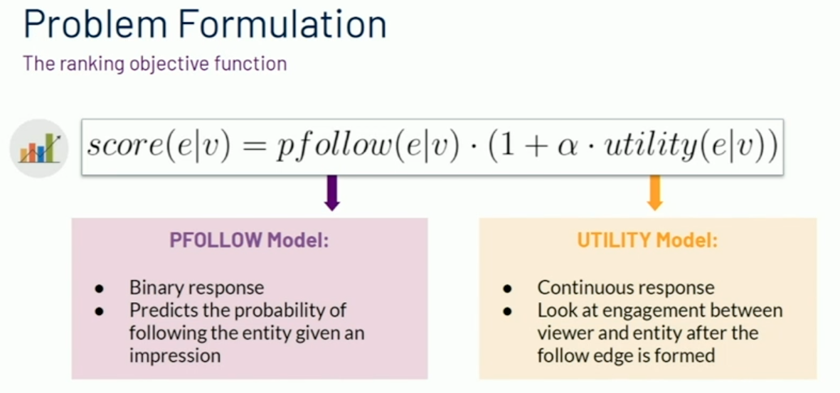
LinkedIn has hundreds of millions of members, and generating recommendations for who to follow is a challenging and data-intensive problem. The goal of this recommendation system is to recommend entities that a member will find interesting (that they’ll actually follow the recommendations) and engaging (that they’ll engage with the recommendations):
LinkedIn has over 690 million members; one immediate task is distinguishing between active members (who have done stuff on LinkedIn lately) and inactive members (who are either new, or registered but don’t use the platform). They handle recommendations differently:
- for active users, create personalized recommendations based on offline, precomputed, member-level data (and real-time contextual recommendations)
- for inactive users, where there’s less data, create segment-based recommendations
The rest of this talk focuses on the somethin
The scoring architecture looks like this:
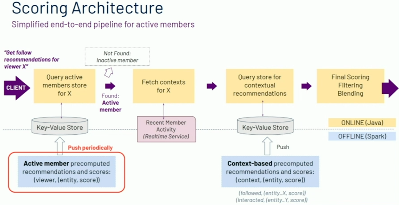
Their features include:
- (few) viewer features, like how often a user will click links on their feed, counts of impressions and interactions, segments like industry, company, skills, etc.
- (moderate) entity features, like the follow-through and unfollow-through rates, feed click-through rates, etc.
- (many) interaction features, like viewer/entity or segment/entity engagement, browsemap scores, embeddings, and many more
Joining millions of active members to millions of entities results in trillions of interaction features; they apply a candidate selection feature that trims this down to “just” hundreds of billions of features. How does this happen?
Generating these features
(1): the naive option is a 3 way Spark join, first on viewerID then on entityID, would be awful; that’d result in two gigantic shuffles of hundreds of terabytes of data while also being highly skewed. This won’t work.
(2): another option is partial scoring using a linear model. Instead of joining all the features together, partially score viewer, entity, and pair features offline, then join the tables of scores instead of the tables of features.
This three-way join is more manageable, but it still has disadvantages; the scoring overhead isn’t great, and there are intermediary steps that they’d like to avoid. You also are forced to score with a linear model (since they’re doing partial scoring on each of viewer, entity, and pair), which is a huge constraint apparently.
(3): the bottlenecks above were the large / wide table of pair features and the skewed entity distribution. They developed a 2D hash-partitioned join for this:
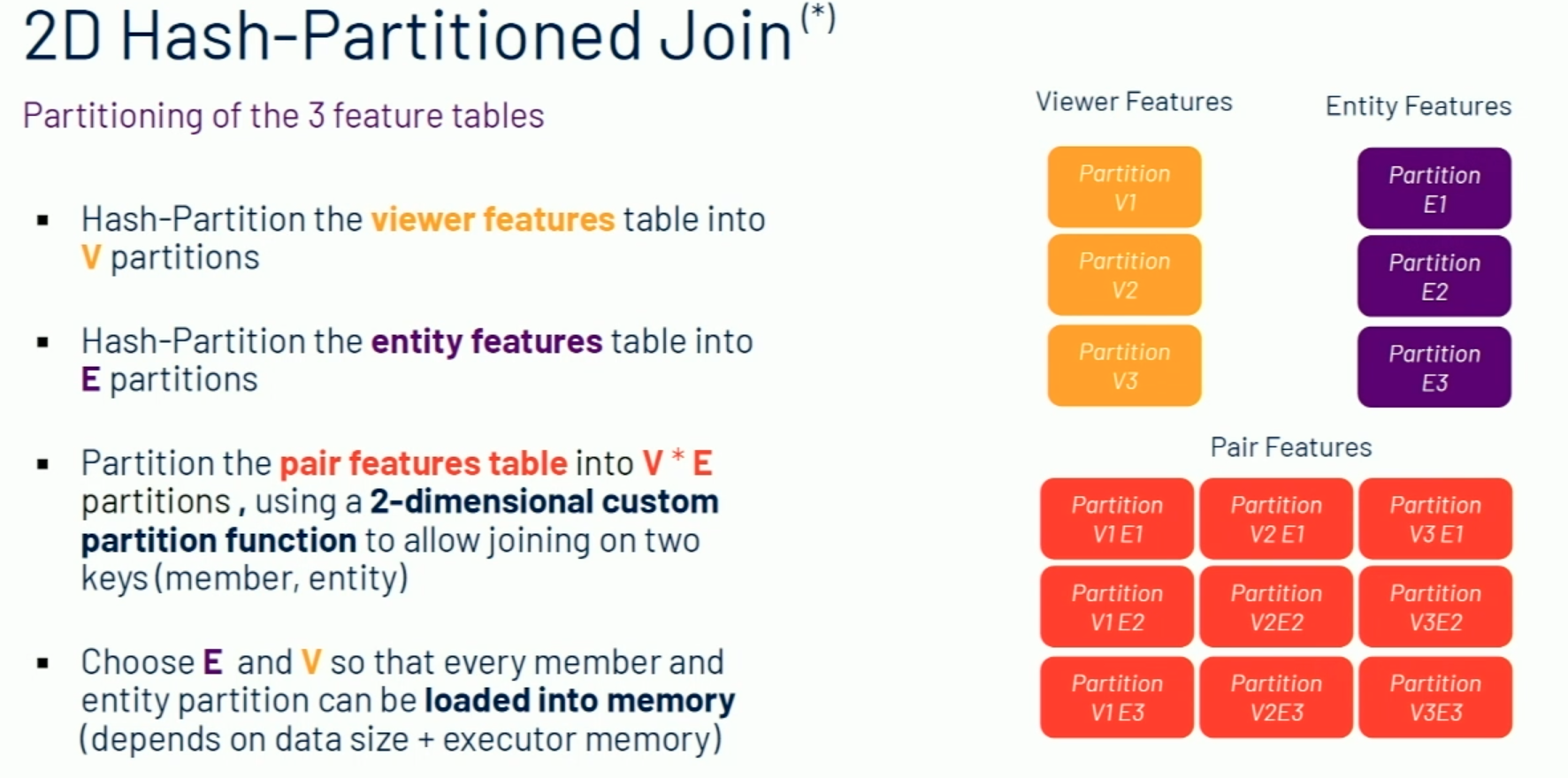
Interesting—I don’t fully understand this, but I think this blog post talks about it in more depth. For a (viewer v, entity e), the viewer will be partitioned into h(v) % V and the entity e(v) % E, putting the pair into h(v) % V*E + h(e) % E, I think.
To do the join, they launch a mapper for each of (V x E) pair partitions, then load the entity partition into memory and the viewer partition into a stream reader. They go through each and merge the three features together, score immediately, and store it to HDFS. Because they score the merged record immediately, they can use a nonlinear model (they use XGBoost), too.
This improved cost by 5x, reduced storage of intermediate outputs by 8x, and (due to the use of XGBoost) improved interest and engagement by 11% and 17% (I think—slide moved away).
Closing thoughts: this was another awesome talk! The slides were incredibly well-designed, and I considered including even more screenshots in this post. The speaker Emilie de Longueau was fantastic and explained this complex topic in an accessible way. The talk went into enough depth to be interesting, but not so much that it lost me.